8 The Logistic Regression Model
Very simply, this model is an extension of the classical regression model. The primary goal of this model is to predict the probability of a binary outcome. Let’s begin with a very simple story. I owe this to Andy Fields, a professor in England. Here’s what he said in one of his books (Discovering Statistics using R).
“Suppose we want to find out which variables are closely related in predicting whether a person is male or female. We might measure laziness, pig-headedness, alcohol consumption, and number of burps that a person does in a day. Using these characteristic variables we can build a logistic regression model and use it to predict whether a new person (who is not part of our original data) is likely to be a male or a female. For example, if we pick a random person and discovered that this person scored high in laziness, pig-headedness, alcohol consumption, and number of burps, then the logistic model might predict, based on this information, that this person is likely to be male. Admittedly, it is unlikely that a researcher would ever be interested in the relationship between flatulence and gender (it is probably too well established by experience to warrant research).”
I hope you had a good laugh while reading the above quote. Now let us look at a real example (a more practical one).
8.1 The Failure of the Linear Model
Suppose you are interested in finding whether a tumor is cancerous or benign and which variables are influential in determining the malignancy of the tumor. The following table shows data from a collection of breast tumors with some characteristics of the tumor and whether they are malignant or benign (indicated by the variable status).
| status | radius | texture | perimeter | area | smoothness | compactness | concavity | concave.points | symmetry | fractal.dimension |
|---|---|---|---|---|---|---|---|---|---|---|
| M | 17.99 | 10.38 | 122.80 | 1001.0 | 0.11840 | 0.27760 | 0.3001 | 0.14710 | 0.2419 | 0.07871 |
| M | 20.57 | 17.77 | 132.90 | 1326.0 | 0.08474 | 0.07864 | 0.0869 | 0.07017 | 0.1812 | 0.05667 |
| M | 19.69 | 21.25 | 130.00 | 1203.0 | 0.10960 | 0.15990 | 0.1974 | 0.12790 | 0.2069 | 0.05999 |
| M | 11.42 | 20.38 | 77.58 | 386.1 | 0.14250 | 0.28390 | 0.2414 | 0.10520 | 0.2597 | 0.09744 |
| M | 20.29 | 14.34 | 135.10 | 1297.0 | 0.10030 | 0.13280 | 0.1980 | 0.10430 | 0.1809 | 0.05883 |
| M | 12.45 | 15.70 | 82.57 | 477.1 | 0.12780 | 0.17000 | 0.1578 | 0.08089 | 0.2087 | 0.07613 |
This dataset is from the UC Irvine machine learning repository. Please see the following webpage for more details of this data: https://archive.ics.uci.edu/ml/datasets/Breast+Cancer+Wisconsin+(Diagnostic)
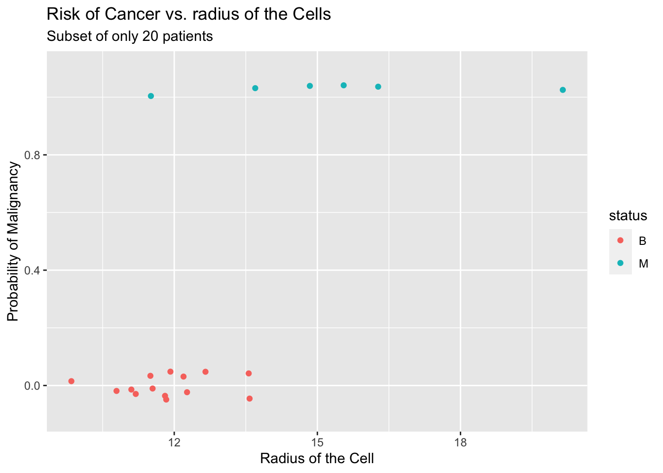
Suppose we want to know the connection between the radius of the cell and malignancy. The relationship of these two variables is shown in the following plot.
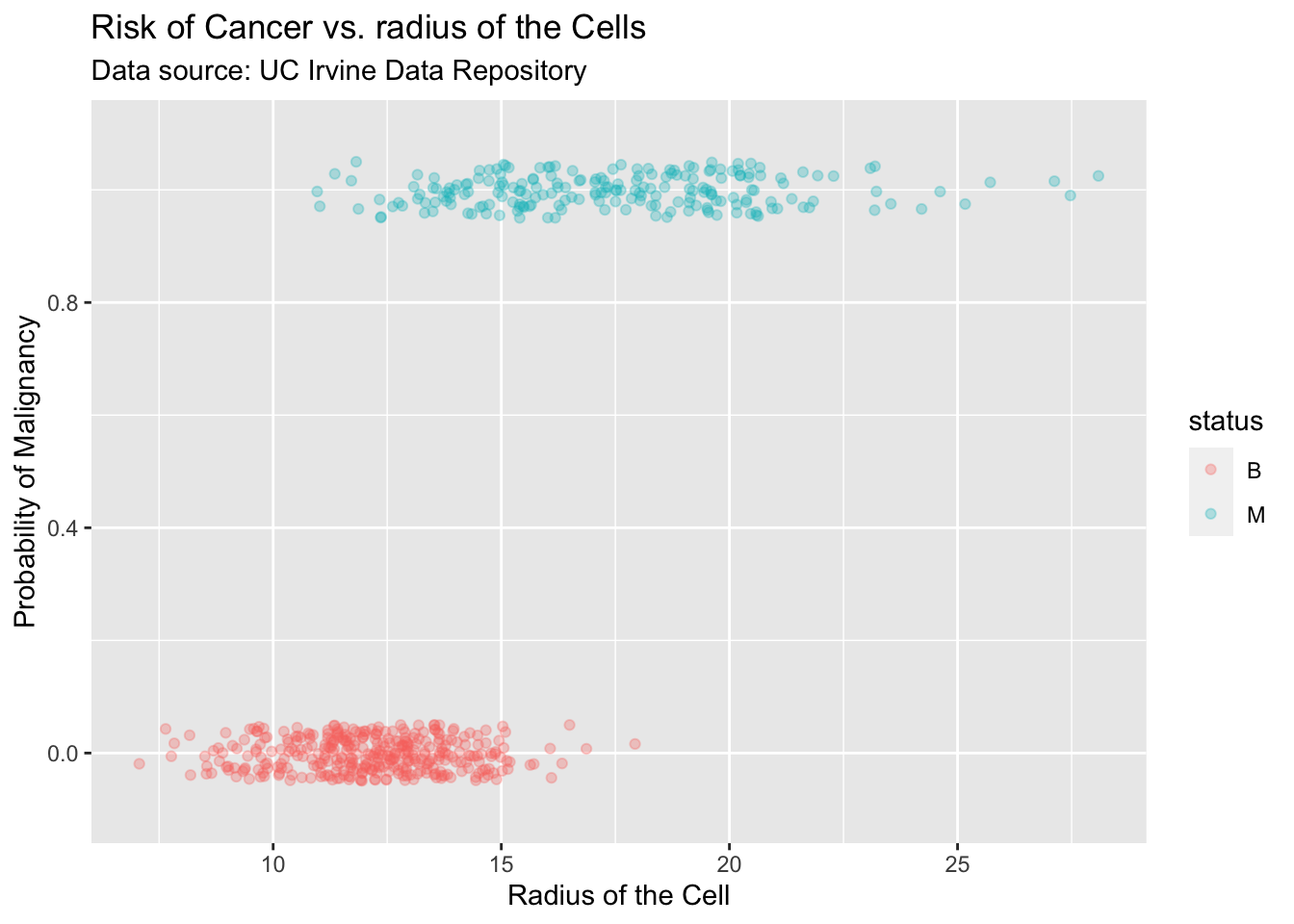
As you can see, cells that are ‘big’ (large radius) tend to be malignant. If we need to utilize this fact to estimate the probability of malignancy of a cell we can create a simple table by partitioning the x-axis into bins and calculate the proportion of malignant cells in each bin. This will give us a very simple estimate (see table below) of the probability of malignancy of a cell and how it is related to the radius.
| Radius | (6,7] | (7,8] | (8,9] | (9,10] | (10,11] | (11,12] | (12,13] | (13,14] | (14,15] | (15,16] | (16,17] | (17,18] | (18,19] | (19,20] |
|---|---|---|---|---|---|---|---|---|---|---|---|---|---|---|
| Proportion | 0 | 0 | 0 | 0 | 0.026 | 0.058 | 0.080 | 0.244 | 0.322 | 0.813 | 0.783 | 0.962 | 1 | 1 |
Plot with Estimates of Probability (local averages)
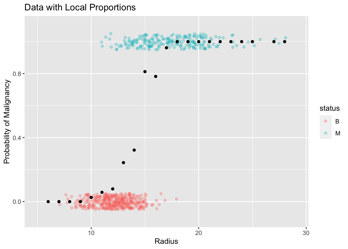
The most important thing to pay attention in the above plot is the range of the local proportions. By definition, all proportions are bounded between [0,1]. Therefore, any model that tries to capture the trend of these proportions has to abide by this restriction. Suppose we try to use the classical simple linear model to capture this trend. You will immediately see why this model is not suitable in this context as shown in the following plot.
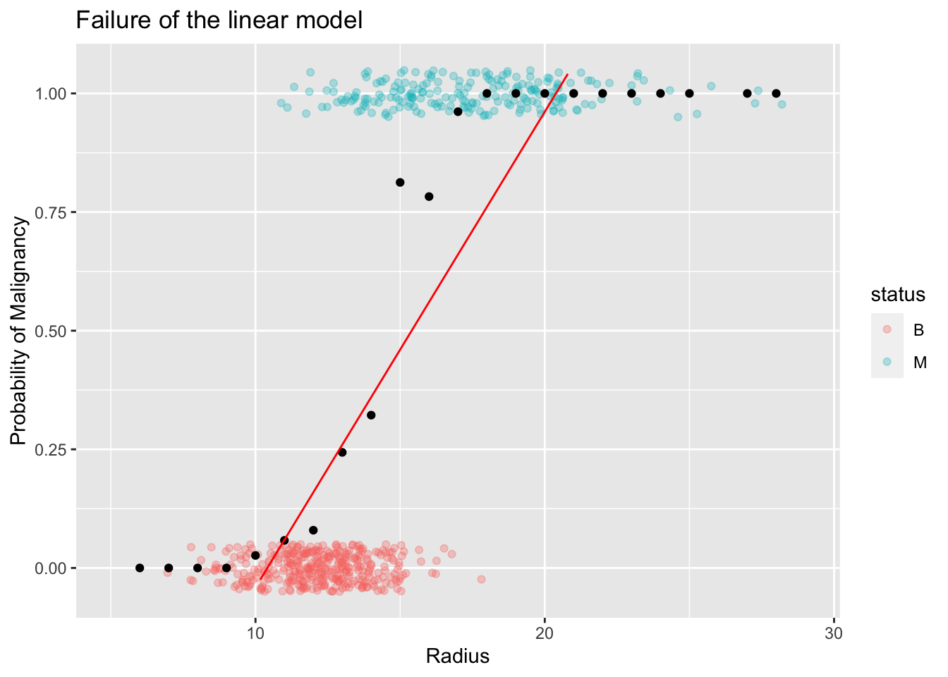
The linear model may produce non-sencical predicted values.  That is, probabilities
bigger than 1 or less than 0.  For example, in this instance, for radius values bigger
than 20 or so you'll end up with predicted probabilities larger than 1!
8.2 Construction of a New Model
How to overcome this issue?
One reasonable approach might be to smooth out the local proportions (black dots) as shown in the following plot.
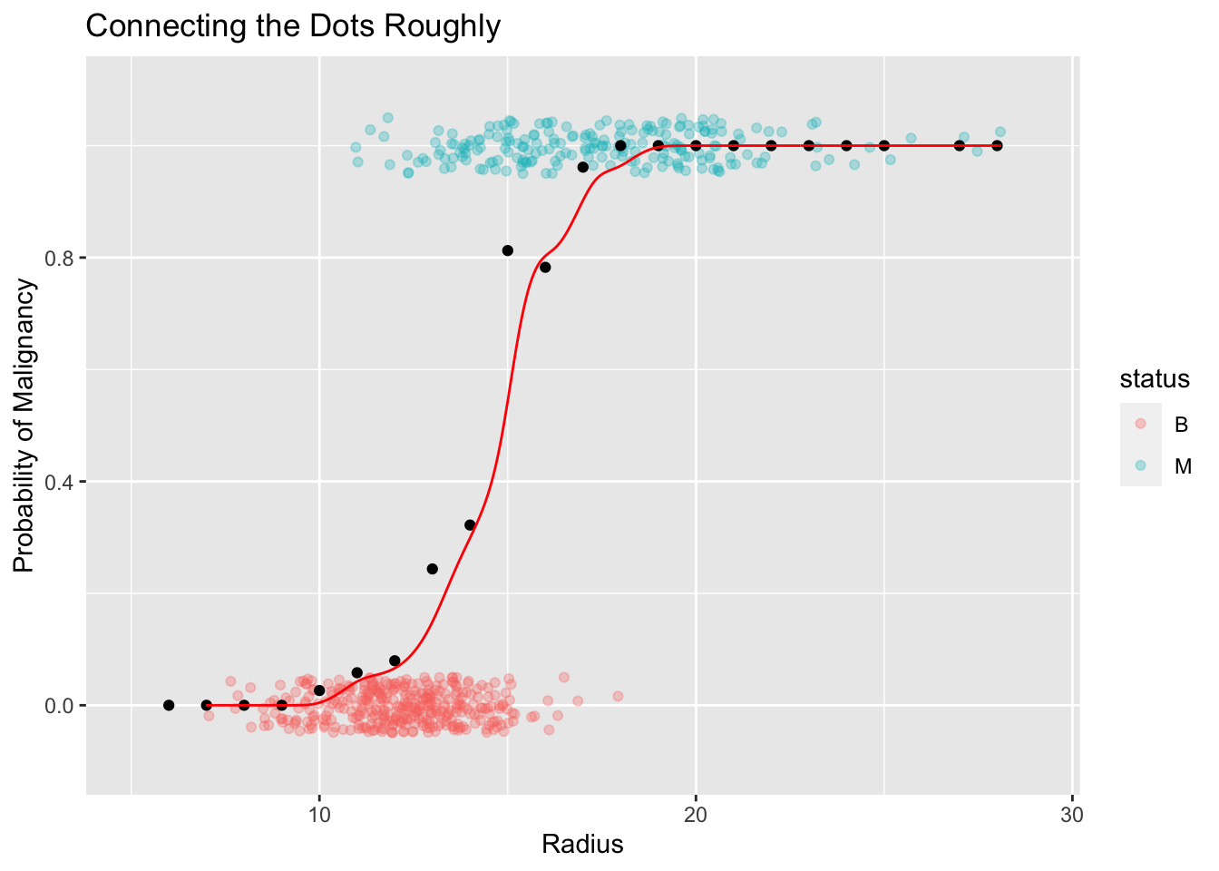
This approach seem to be quite good. But it has some shortcomings.
On rare occasions we might end up with probabilities bigger than 1 (or less than 0)
It does not allow us to adequately quantify the effect of radius on the probability of malignancy.
Let’s unpack issue number 2 above. Consider the following dialog:
You: I’m not sure what you mean in issue number 2 above.
Me:: What I mean by this is we are unable to answer questions like, “how much the probability might increase (or decrease) for different values of the \(X\) variable?”.
You: Yes we can. We can look at the smooth line and eyeball (roughly estimate) the difference in probabilities.
Me: Sure, that’s true. But it is a very rough estimate. If you are dealing with a life threatening situation like malignancy of a tumor, don’t you think you’d rather have a more precise method than just eyeballing?
You: I guess that’s reasonable.
Me: We need something like the simple linear regression model \(\hat Y = a + bX\) where the “effect” of \(X\) is adequately captured by a model parameter (like the slope of the line). The coefficient of \(X\), \(b\), is a summary value of the “effect” of \(X\) on the response \(Y\). We need a similar model that can adequately capture (and summarize) the relationship between \(X\) and \(Y\).
You: So how do we build such a model?
Me: That’s what we are going to learn in the rest of this chapter. Let’s dive in.
What we need is a model which does not exceed 1 for large \(X\) values and which does not go below 0 for small \(X\) values. There are several mathematical functions that obey these restrictions. One such function is the Logistic function. The mathematical equation for this function and its plot is given below: \[ f(x) = \frac{e^x}{1 + e^x} \]
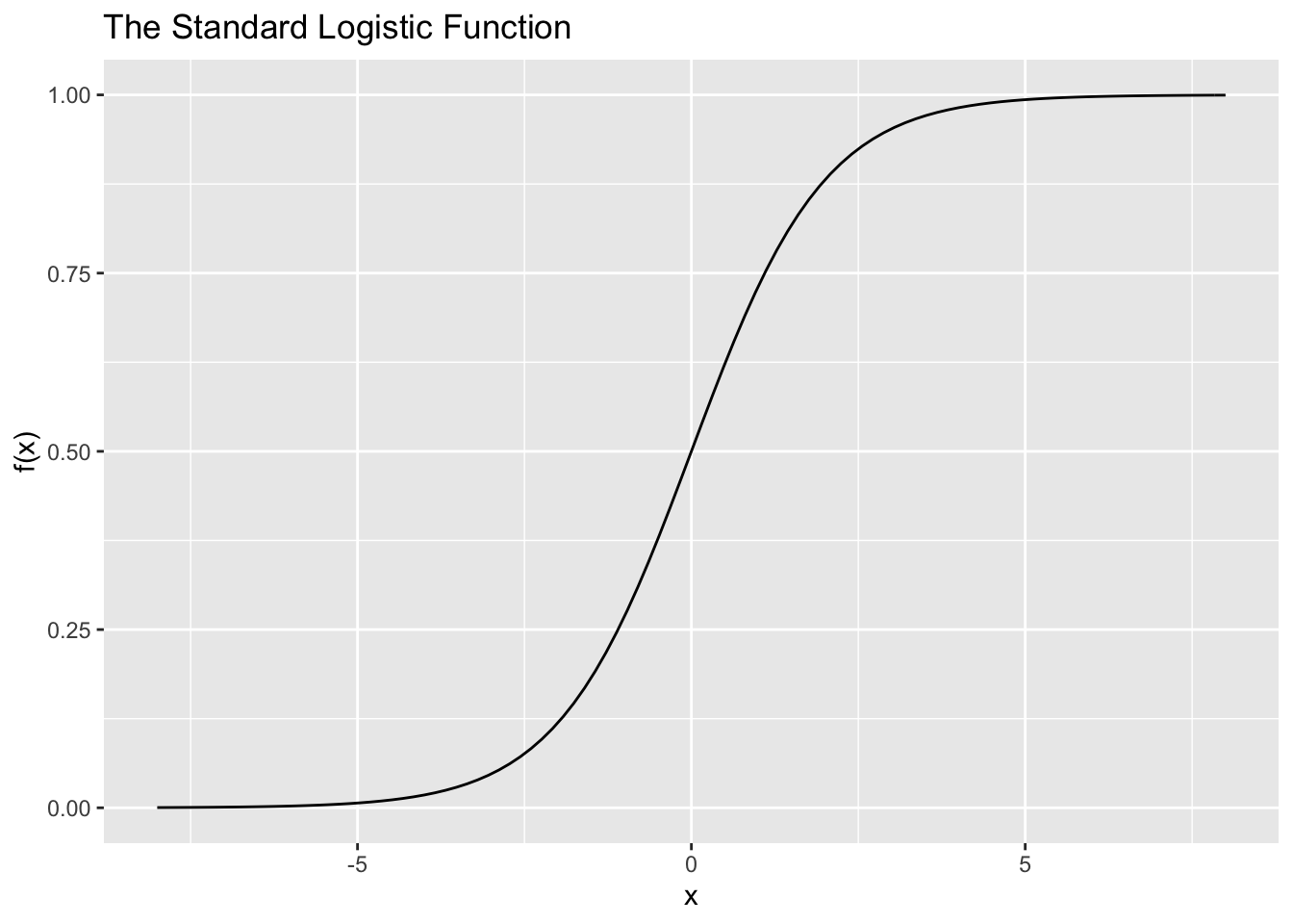
This function seems to be good solution for our problem. Let’s try to fit this curve to our data.
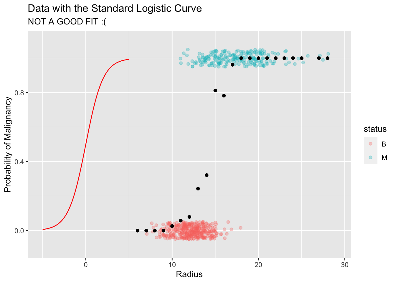
As you can see, the curve does not fit the data at all. The main issue is that it is centered at the wrong place.
Q: How to shift this curve to the right?

Answer:  We need some type of an "intercept" parameter similar to what we have in a linear model.
Let’s shift this curve to the right by 15 units. The equation of this new curve and its corresponding plot is given below:
\[ f(x) = \frac{e^{-15 + x}}{1 + e^{-15 + x}} \]
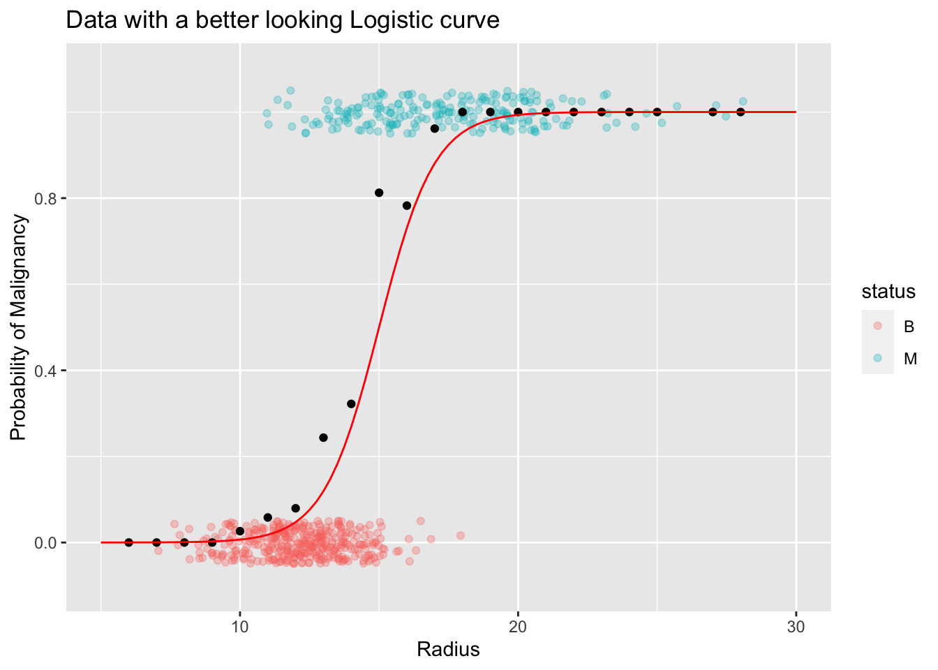
Note: You might wonder why we have -15 instead of 15. This is not an error. In fact, this is one of your HW problems. Hint: Think about a much simpler function like \(f(x) = x^2\). How would you shift this, say 15 units to the right (x-direction)?
As the above plot shows this new curve seem to fit the data really well. Perhaps, we can adjust the the steepness of the curve to fit the data points (local proportions) in the mid section. We can do that by introducing a parameter (like a “slope”) to the curve as shown in the following equation and the plot:
\[ f(x) = \frac{e^{-15 + 1.05x}}{1 + e^{-15 +1.05x}} \]
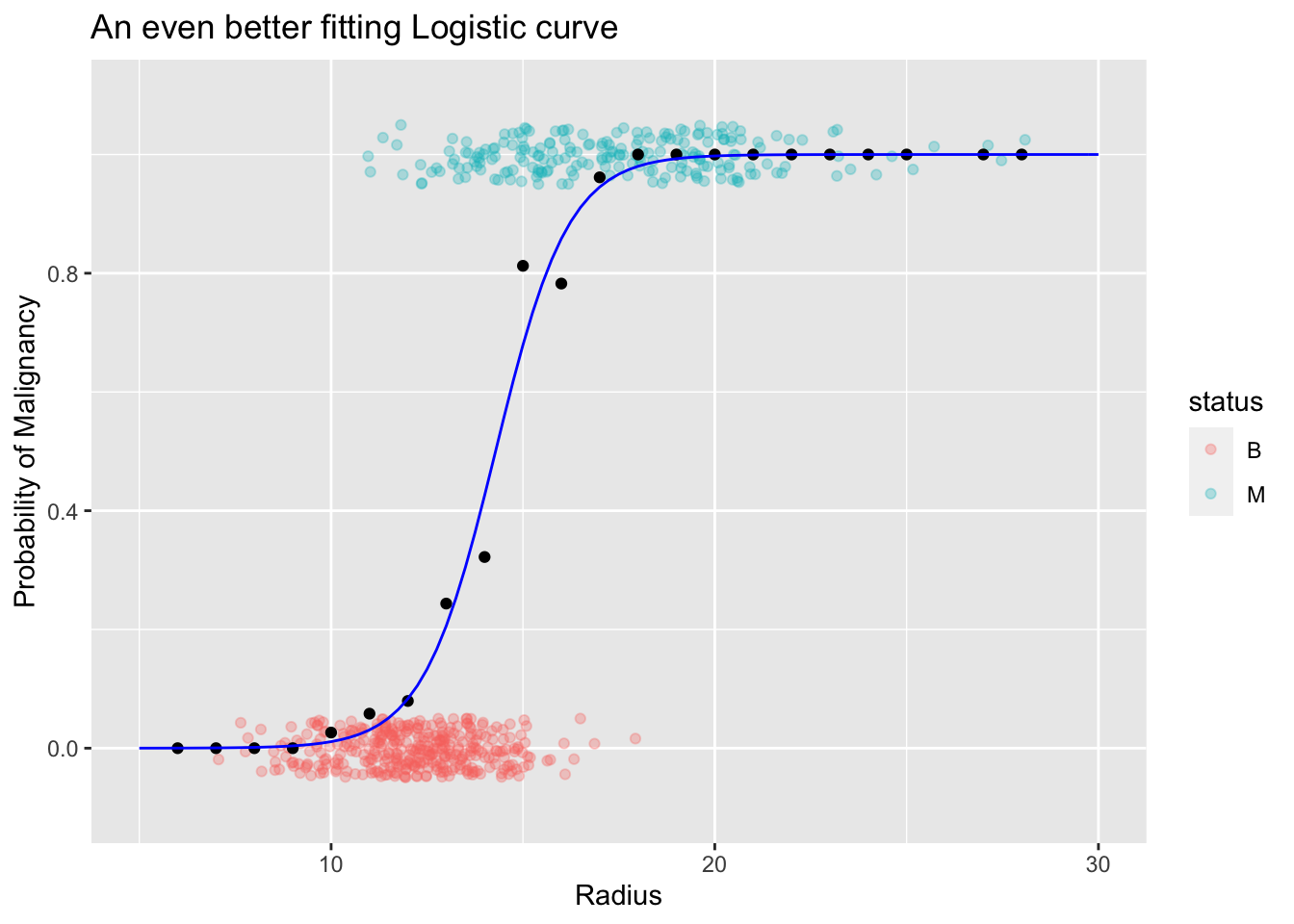
Now you might be wondering whether we have to use this trial an error approach in fitting this curve to the data. The answer is: No. We have a systematic way to find the location and the shape of the logistic function. That is the focus in the next section.
8.3 Fitting a Logistic Model
The logistic model that we fit to the data has the following general form:
\[ f(x) = \frac{e^{a + bx}}{1 + e^{a + bx}} \]
The coefficients \(a\) and \(b\) are called model parameters. As you saw earlier these two coefficients are like two dials which controls two attributes of the curve.
| Coefficient | Role |
|---|---|
| \(a\) | Controls the location of the curve. It centers the curve where the data is. |
| \(b\) | Controls the steepness (shape) of the curve. |
Similar to what we did earlier (using trial and error), our goal is to find the “curve of best fit”. The technique we use is called the maximum likelihood estimation. Let’s try to get our feet wet on this new concept.
Maximum Likelihood Estimation
This is one of the celebrated and time tested techniques in statistics. It is an intuitive method with many desirable properties and it is easy to implement using any statistical software. Let’s look at some toy examples to understand the fundamentals behind this technique.
Example 1:
Cookie jar, number of chocolate chip cookies, \(\theta\), is either 6 or 2. That is, the set of possible values for \(\theta\) is \(\{6,2\}\). We call this set the parameter space of \(\theta\).
\(\theta = \{6,2\}\)
Now suppose you picked a one cookie at random and found out that it is a chocolate chip cookie. Based on this sample (`evidence’) what is the most likely value of \(\theta\)?
If you guessed 6 you’re correct. Our intuition tells us that it is more likely that we get a chocolate-chip cookie if \(\theta\) were 6 than if \(\theta\) were 2.
We can make this argument more precise by calculating the likelihood of getting a chocolate-chip cookie for the two values of \(\theta\).
\[P[ X = CC\ cookie\ |\ \theta = 6] = 6/10 \]
\[P[ X = CC\ cookie \ |\ \theta = 2] = 2/10 \]
Based on this sample of size 1, our choice for \(\theta\) is 6.
Let’s make it more interesting. What if we draw two cookies without replacement and found out that both of them are NOT chocolate chip cookies. Now what is your guess for the value of \(\theta\) ?
Again, we can calculate the probabilities for this outcome under the two scenarios \(\theta = 6\) and \(\theta = 2\).
\[P[ X_1 = NotCC, X_2 = NotCC \ |\ \theta = 6] = (4/10) . (3/9) = 0.13 \]
\[P[ X_1 = NotCC, X_2 = NotCC \ |\ \theta = 2] = (8/10) . (7/9) = 0.80 \]
Now based on this sample of size 2, our choice for \(\theta\) is 2.
I hope now you’ll start to see a pattern. We pick a value for the parameter \(\theta\) based on the likelihood of the observed (realized) outcomes in our sample. That is, we choose the value (of \(\theta\)) to make our observed outcome most likely. This is the principle behind maximum likelihood estimation. Let’s look at another example.
Example 2:
Suppose I give you a coin from my country Sri Lanka and told you that this is an unbiased coin. Knowing who I am, you might suspect whether I’m being truthful about this coin. Here is a picture of my coin.

Figure 8.1: Two sides of a Sri Lankan Coin. We label the side with the emblem (left picture) as heads.
Suppose you are interested in the unbiased nature of my coin. If we denote \(\theta\) as the probability of heads, then \(\theta\) could be any value between [0,1]. If I’m being truthful, you’d say \(\theta = 0.5\) (unbiased coin). You decided to test my claim of unbiasedness by flipping it 10 times. Suppose after 10 flips you got the following sequence of heads and tails. \[HHHTHHTTHH\]
Based on this evidence, what is the most likely value of \(\theta\)?
You might guess \(\theta\) to be 0.7. If you did, you effectively found the maximum likelihood estimate of \(\theta\). Recall that we choose the value of \(\theta\) that maximizes the likelihood of the observed (realized) sample. You might wonder, could there be any other value (other than 0.7) which yields a higher likelihood for this observed outcome \(HHHTHHTTHH\). Let’s check with some other values of \(\theta\).
| \(\theta\) | Probability of \(HHHTHHTTHH\) outcome |
|---|---|
| 0.1 | 0.00000 |
| 0.2 | 0.00000 |
| 0.3 | 0.00007 |
| 0.4 | 0.00035 |
| 0.5 | 0.00097 |
| 0.6 | 0.00179 |
| 0.7 | 0.00222 |
| 0.8 | 0.00167 |
| 0.9 | 0.00047 |
How did I calculate the above probabilities?
Answer
If we denote the probability of heads as \(\theta\) and denote \(y_i=1\) if the \(i^{th}\) flip is a head and \(y_i=0\) if the \(i^{th}\) flip is a tails, then we can write the likelihood of the observed outcome as follows:
\[P[HHHTHHTTHH] = \prod_{i=1}^{10} \theta^{y_i}(1-\theta)^{1-y_i} = \theta^7(1-\theta)^3\]
Note 1: The symbol \(\prod_{i=1}^{10}\) is the product operator. It is a notation that we use to simplify things.
Note 2: The above probability is a function of \(\theta\). We call this function, the likelihhod function, \(L(\theta)\).
Then, by plugging in values \(0.1,0.2, \ldots, 0.9\) to the above equation yields the corresponding probabilities.
In fact, we can be even more precise. If you plot the above function \(L(\theta\)) you’ll get the following plot:
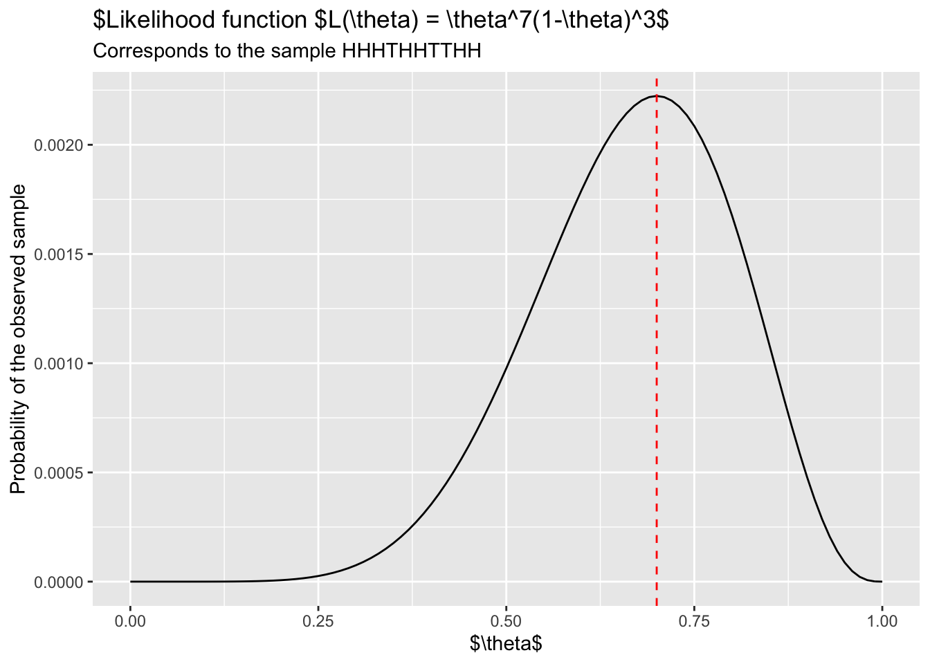
As shown in the above plot, the maximum of the likelihood function \(L(\theta)\) occurs at \(\theta = 0.7\).
Example 3:
In this example, let’s extend the intuition of the maximum likelihood estimation to the logistic model. Consider the following simple dataset, a subset of breast cancer dataset that you saw in earlier examples.
How to use the Maximum Likelihood method to find the correct logistic curve?
Recall my Sri Lankan coin flipping example. The breast cancer data can be thought of as a special coin flipping experiment where the probability of malignancy, \(p\), is dependent on the radius of the cell. That is, \(p\) is a function of radius. In particular, we claim that this probability can be modeled by a logistic curve. That is,
\[ p(radius) = \frac{e^{a + b(radius)}}{1 + e^{a + b(radius)}}\]
If you look at the above plot you can see that there are 6 malignant cases and 14 benign cases. So we can write down the likelihood of observing the outcome \([\ MMMMMM\ BBBBBBBBBBBBBB \ ]\). If we denote \(y_i=1\) for malignant cases and \(y_i=0\) for benign cases, we can write the required probability as follows:
\[P[\ MMMMMM\ BBBBBBBBBBBBBB \ ] = \prod_{i=1}^{20} p(radius_i)^{y_i}(1-p(radius_i))^{1-y_i} \]
Note 1: The symbol \(\prod_{i=1}^{20}\) is the product operator. It is a notation that we use to simplify things.
Note 2: The outcome of this expression is a mess. But, if you look at it carefully it is a simple function of 3 things: The model parameters \(a\) and \(b\), and the radius values (data) of the 20 patients.
In order to get a better sense, take a look at the plot below. It is the plot of the likelihood for this dataset. Rotate the plot using your mouse to see where the likelihood is maximized.
| term | estimate | std.error | statistic | p.value |
|---|---|---|---|---|
| (Intercept) | -16.823 | 7.313 | -2.300 | 0.021 |
| radius | 1.221 | 0.555 | 2.202 | 0.028 |